
© 2013, NVIDIA CORPORATION. All rights reserved.
Code and text by Sean Baxter, NVIDIA Research.
(Click here for license. Click here for contact information.)
Load-balancing search is a specialization of vectorized sorted search. It coordinates output items with the input objects that generated them. The CTA load-balancing search is a fundamental tool for partitioning irregular problems.
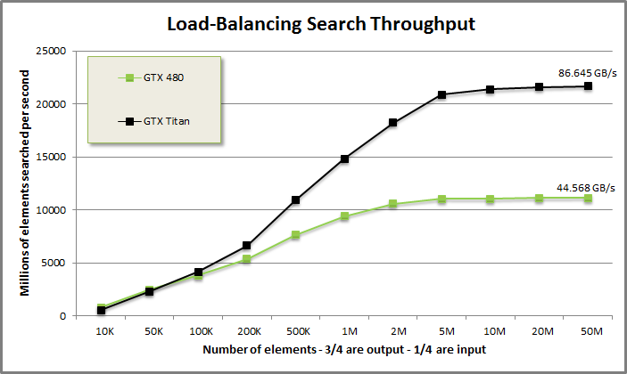
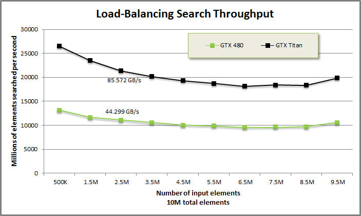
Load-balancing search benchmark from benchmarkloadbalance/benchmarkloadbalance.cu
Load-balancing search demonstration from tests/demo.cu
void DemoLBS(CudaContext& context) {
	printf("\n\nLOAD-BALANCING SEARCH DEMONSTRATION:\n\n");

	// Use CudaContext::GenRandom to generate work counts between 0 and 5.
	int N = 50;
	MGPU_MEM(int) counts = context.GenRandom<int>(N, 0, 5);

	printf("Object counts\n");
	PrintArray(*counts, "%4d", 10);

	// Scan the counts.
	int total = Scan(counts->get(), N, context);
	printf("\nScan of object counts:\n");
	PrintArray(*counts, "%4d", 10);
	printf("Total: %4d\n", total);

	// Allocate space for the object references and run load-balancing search.
	MGPU_MEM(int) refsData = context.Malloc<int>(total);
	LoadBalanceSearch(total, counts->get(), N, refsData->get(), context);

	printf("\nObject references:\n");
	PrintArray(*refsData, "%4d", 10);
}
LOAD-BALANCING SEARCH DEMONSTRATION:
Object counts
0: 0 3 5 2 1 3 1 5 4 5
10: 2 5 4 0 2 3 1 4 0 5
20: 4 3 2 4 2 4 3 3 0 3
30: 1 4 4 4 4 2 0 3 0 5
40: 0 0 0 0 2 2 3 0 4 4
Scan of object counts:
0: 0 0 3 8 10 11 14 15 20 24
10: 29 31 36 40 40 42 45 46 50 50
20: 55 59 62 64 68 70 74 77 80 80
30: 83 84 88 92 96 100 102 102 105 105
40: 110 110 110 110 110 112 114 117 117 121
Total: 125
Object references:
0: 1 1 1 2 2 2 2 2 3 3
10: 4 5 5 5 6 7 7 7 7 7
20: 8 8 8 8 9 9 9 9 9 10
30: 10 11 11 11 11 11 12 12 12 12
40: 14 14 15 15 15 16 17 17 17 17
50: 19 19 19 19 19 20 20 20 20 21
60: 21 21 22 22 23 23 23 23 24 24
70: 25 25 25 25 26 26 26 27 27 27
80: 29 29 29 30 31 31 31 31 32 32
90: 32 32 33 33 33 33 34 34 34 34
100: 35 35 37 37 37 39 39 39 39 39
110: 44 44 45 45 46 46 46 48 48 48
120: 48 49 49 49 49//////////////////////////////////////////////////////////////////////////////// // kernels/loadbalance.cuh // LoadBalanceSearch is a special vectorized sorted search. Consider bCount // objects that generate a variable number of work items, with aCount work // items in total. The caller computes an exclusive scan of the work-item counts // into b_global. // indices_global has aCount outputs. indices_global[i] is the index of the // object that generated the i'th work item. // Eg: // work-item counts: 2, 5, 3, 0, 1. // scan counts: 0, 2, 7, 10, 10. aCount = 11. // // LoadBalanceSearch computes the upper-bound of counting_iterator<int>(0) with // the scan of the work-item counts and subtracts 1: // LBS: 0, 0, 1, 1, 1, 1, 1, 2, 2, 2, 4. // This is equivalent to expanding the index of each object by the object's // work-item count. MGPU_HOST void LoadBalanceSearch(int aCount, const int* b_global, int bCount, int* indices_global, CudaContext& context);
Consider an array of objects O[i] (i < N) that each generate a non-negative variable number of work-items counts[i]. The sum of counts is M:
Work-item counts:
    0:     1    2    4    0    4    4    3    3    2    4
   10:     0    0    1    2    1    1    0    2    2    1
   20:     1    4    2    3    2    2    1    1    3    0
   30:     2    1    1    3    4    2    2    4    0    4

Exc-scan of counts:
    0:     0    1    3    7    7   11   15   18   21   23
   10:    27   27   27   28   30   31   32   32   34   36
   20:    37   38   42   44   47   49   51   52   53   56
   30:    56   58   59   60   63   67   69   71   75   75

Inc-scan of counts:
    0:     1    3    7    7   11   15   18   21   23   27
   10:    27   27   28   30   31   32   32   34   36   37
   20:    38   42   44   47   49   51   52   53   56   56
   30:    58   59   60   63   67   69   71   75   75   79

Total work-items: 79
It is simple to calculate the range of work-items that each object creates. We exclusive scan the work-item counts: these are the 'begin' indices for each object's run of outputs. The 'end' indices, if desired, are the inclusive scan of the objects' counts, or the exclusive scan plus the counts.
Consider this mapping of object counts into work-items a forward transformation. The corresponding inverse transformation, which maps work-items into the objects that generated them, is not as straight-forward.
Lower-bound search of work-items into exc-scan of counts:
    0:     0    1    2    2    3    3    3    3    5    5
   10:     5    5    6    6    6    6    7    7    7    8
   20:     8    8    9    9   10   10   10   10   13   14
   30:    14   15   16   18   18   19   19   20   21   22
   40:    22   22   22   23   23   24   24   24   25   25
   50:    26   26   27   28   29   29   29   31   31   32
   60:    33   34   34   34   35   35   35   35   36   36
   70:    37   37   38   38   38   38   40   40   40

Lower-bound search of work-items into inc-scan of counts:
    0:     0    0    1    1    2    2    2    2    4    4
   10:     4    4    5    5    5    5    6    6    6    7
   20:     7    7    8    8    9    9    9    9   12   13
   30:    13   14   15   17   17   18   18   19   20   21
   40:    21   21   21   22   22   23   23   23   24   24
   50:    25   25   26   27   28   28   28   30   30   31
   60:    32   33   33   33   34   34   34   34   35   35
   70:    36   36   37   37   37   37   39   39   39
The 40 objects generated 79 work-items. Running a lower-bound search from each work-item index (i.e. keys from 0 to 78) on either the exclusive or inclusive scan of object counts doesn't quite work—the indices in red indicate mismatches. What does work is taking the upper-bound of work-item indices with the exclusive scan of the counts and subtracting one:
Work-item counts:
    0:     1    2    4    0    4    4    3    3    2    4
   10:     0    0    1    2    1    1    0    2    2    1
   20:     1    4    2    3    2    2    1    1    3    0
   30:     2    1    1    3    4    2    2    4    0    4

Exc-scan of counts:
    0:     0    1    3    7    7   11   15   18   21   23
   10:    27   27   27   28   30   31   32   32   34   36
   20:    37   38   42   44   47   49   51   52   53   56
   30:    56   58   59   60   63   67   69   71   75   75

Load-balancing search:
    0:     0    1    1    2    2    2    2    4    4    4
   10:     4    5    5    5    5    6    6    6    7    7
   20:     7    8    8    9    9    9    9   12   13   13
   30:    14   15   17   17   18   18   19   20   21   21
   40:    21   21   22   22   23   23   23   24   24   25
   50:    25   26   27   28   28   28   30   30   31   32
   60:    33   33   33   34   34   34   34   35   35   36
   70:    36   37   37   37   37   39   39   39   39

Work-item rank (i - excscan[LBS[i]]):
    0:     0    0    1    0    1    2    3    0    1    2
   10:     3    0    1    2    3    0    1    2    0    1
   20:     2    0    1    0    1    2    3    0    0    1
   30:     0    0    0    1    0    1    0    0    0    1
   40:     2    3    0    1    0    1    2    0    1    0
   50:     1    0    0    0    1    2    0    1    0    0
   60:     0    1    2    0    1    2    3    0    1    0
   70:     1    0    1    2    3    0    1    2    3
The load-balancing search providhes each work-item with the index of the object that generated it. The object index can then be used to find the work-item's rank within the generating object. For example, work-item 10 in the figure above was generated by object 4 (see element 10 in the load-balancing search). The scan of counts at position 4 is 7. The difference between the work-item's index (10) and the object's scan (7) is the work-item's rank within the object: 10 - 7 = 3.
CPULoadBalanceSearch from benchmarkloadbalance/benchmarkloadbalance.cu
void CPULoadBalanceSearch(int aCount, const int* b, int bCount, int* indices) {
	int ai = 0, bi = 0;
	while(ai < aCount || bi < bCount) {
		bool p;
		if(bi >= bCount) p = true;
		else if(ai >= aCount) p = false;
		else p = ai < b[bi];	// aKey < bKey is upper-bound condition.

		if(p) indices[ai++] = bi - 1;	// subtract 1 from the upper-bound.
		else ++bi;
	}
}
The serial implementation for the load-balancing search is very simple. We only support integer types and the A array is just the sequence of natural numbers. When written this way it's clear that the load-balancing search is immediately parallelizable, and as both input arrays are monotonically non-decreasing, it is in fact a special case of the vectorized sorted search from the previous page.
Important: Load-balancing search is kind of scan inverse. It operates on scanned work-item counts and returns the index of the object that generated each work-item. It's more accurate to consider the load-balancing search as an idiom or pattern rather than an algorithm. It's not a step-by-step procedure and it's not intended to directly solve problems. Rather, the load-balancing search is a concept that helps the programmer better understand scheduling in problems with irregular parallelism.
CTALoadBalance is a very light-weight operator. It can be included at the top of kernels as boilerplate, transforming thread IDs (or global output IDs) into the coordinate space of generating objects. The next two algorithms covered, Interval Move and relational join, use this embedded form of load-balancing search.
You'll usually need to call MergePathPartitions in the host code immediately prior to launching a kernel that uses intra-CTA load-balancing search. This global search runs an upper-bound binary search to find the intersection of each CTA's cross-diagonal with the Merge Path curve defined by the set of all work-item indices (a counting_iterator<int>) and the exclusive scan of work-item counts.
include/device/ctaloadbalance.cuh
template<int VT, bool RangeCheck>
MGPU_DEVICE void DeviceSerialLoadBalanceSearch(const int* b_shared, int aBegin,
	int aEnd, int bFirst, int bBegin, int bEnd, int* a_shared) {

	int bKey = b_shared[bBegin];

	#pragma unroll
	for(int i = 0; i < VT; ++i) {
		bool p;
		if(RangeCheck)
			p = (aBegin < aEnd) && ((bBegin >= bEnd) || (aBegin < bKey));
		else
			p = aBegin < bKey;

		if(p)
			// Advance A (the needle).
			a_shared[aBegin++] = bFirst + bBegin;
		else
			// Advance B (the haystack).
			bKey = b_shared[++bBegin];
	}
}
We'll start with the serial loop DeviceSerialLoadBalanceSearch, a GPU treatment of CPULoadBalanceSearch. The interval of scan elements available to the thread, b_shared, are passed to the function in shared memory. Elements of the A array are output (work-item) indices and are generated directly from the interval range.
Because the A inputs take no space in shared memory, and because we emit one output per A input, we store search results directly to shared memory rather than to register array. This is a break from the other routines in this library, where we gather sources from shared memory and keep temporary outputs in register, synchronize, then store back to shared memory to conserve space. The sequential nature of the A inputs lets us store the upper-bound - 1 directly into shared memory, simplifying the routine.
Like vectorized sorted search, full tiles that load a halo element at the end of the CTA's B interval can elide range checking. The nominal form of DeviceSerialLoadBalanceSearch makes only a single comparison (aBegin < bKey) per iteration, giving us a very lightweight and low-latency function.
include/device/ctaloadbalance.cuh
template<int NT, int VT>
MGPU_DEVICE int4 CTALoadBalance(int destCount, const int* b_global,
	int sourceCount, int block, int tid, const int* mp_global,
	int* indices_shared, bool loadPrecedingB) {

	int4 range = ComputeMergeRange(destCount, sourceCount, block, 0, NT * VT,
		mp_global);

	int a0 = range.x;
	int a1 = range.y;
	int b0 = range.z;
	int b1 = range.w;

	if(loadPrecedingB) {
		if(!b0) loadPrecedingB = false;
		else --b0;
	}

	bool extended = a1 < destCount && b1 < sourceCount;
	int aCount = a1 - a0;
	int bCount = b1 - b0;

	int* a_shared = indices_shared;
	int* b_shared = indices_shared + aCount;

	// Load the b values (scan of work item counts).
	DeviceMemToMemLoop<NT>(bCount + (int)extended, b_global + b0, tid,
		b_shared);

	// Run a merge path to find the start of the serial merge for each thread.
	int diag = min(VT * tid, aCount + bCount - (int)loadPrecedingB);
	int mp = MergePath<MgpuBoundsUpper>(mgpu::counting_iterator<int>(a0),
		aCount, b_shared + (int)loadPrecedingB, bCount - (int)loadPrecedingB,
		diag, mgpu::less<int>());

	int a0tid = a0 + mp;
	int b0tid = diag - mp + (int)loadPrecedingB;

	// Subtract 1 from b0 because we want to return upper_bound - 1.
	if(extended)
		DeviceSerialLoadBalanceSearch<VT, false>(b_shared, a0tid, a1, b0 - 1,
			b0tid, bCount, a_shared - a0);
	else
		DeviceSerialLoadBalanceSearch<VT, true>(b_shared, a0tid, a1, b0 - 1,
			b0tid, bCount, a_shared - a0);
	__syncthreads();

	return make_int4(a0, a1, b0, b1);
}
CTALoadBalance is the standard CTA-entry point for load-balancing search and a function we've demonstrated back in the introduction.
An upper-bound MergePath search divides input arrays A (the natural numbers) and B (the scan of counts) into distinct, non-overlapping ranges. ComputeMergeRange returns the tuple (a0, a1, b0, b1) of input intervals. Scan offsets are loaded into shared memory with DeviceMemToMemLoop, a device function that cooperatively loads intervals that are expected to be much smaller than NV elements.
MergePath<MgpuBoundsUpper> is called on counting_iterator<int>(0) to divide the input domains into equal-size partitions. DeviceSerialLoadBalance sequentially traverses the inputs and stores search indices to the start of shared memory, where the caller expects to see them returned.
A array:
    0:     0    1    2    3    4    5    6    7    8    9
   10:    10   11   12   13   14   15   16   17   18   19
   20:    20   21   22   23   24   25   26   27   28   29
   30:    30   31   32   33   34   35   36   37   38   39
   40:    40   41   42   43   44   45   46   47   48   49
   50:    50   51   52   53   54   55   56   57   58   59
   60:    60   61   62   63   64   65   66   67   68   69
   70:    70   71   72   73   74   75   76   77   78

B array (Exc-scan of counts):
    0:     0    1    3    7    7   11   15   18   21   23
   10:    27   27   27   28   30   31   32   32   34   36
   20:    37   38   42   44   47   49   51   52   53   56
   30:    56   58   59   60   63   67   69   71   75   75

Divide into 4 equal partitions:
Tile 0: A = ( 0, 21)  B = ( 0,  9)
Tile 1: A = (21, 38)  B = ( 9, 22)
Tile 2: A = (38, 58)  B = (22, 31)
Tile 3: A = (58, 79)  B = (31, 40)

Load-balancing search:
    0:     0    1    1    2    2    2    2    4    4    4
   10:     4    5    5    5    5    6    6    6    7    7
   20:     7    8    8    9    9    9    9   12   13   13
   30:    14   15   17   17   18   18   19   20   21   21
   40:    21   21   22   22   23   23   23   24   24   25
   50:    25   26   27   28   28   28   30   30   31   32
   60:    33   33   33   34   34   34   34   35   35   36
   70:    36   37   37   37   37   39   39   39   39
There is a minor complication regarding the ranges of data to load. Consider dividing the sample objects into four evenly-sized parts. Tile 0 loads, notionally, (0, 21) from A and (0, 9) from B. Tile 1 loads (21, 38) from A and (9, 22) from B; etc. If a CTA only wishes to compute the load-balancing search, adhering to this non-overlapping coverage is adequete, as we know from dealing with vectorized sorted search.
If, on the other hand, the caller wishes to compute the rank of each work-item within its generating object in addition to that object's index, a modification is required. Take, for example, the tile that loads the elements in red. Its first work-item (item 21) is generated by object 8 (see index 21 in the load-balancing search). We try to compute the rank of item 21 by looking up element 8 of the scan of counts, but that element is mapped into a different tile! This is due to the upper-bound Merge Path consuming elements of B (the scan) before consuming equal elements of A (the work-item indices).
We rectify this problem by simply loading the preceding element of B, if available. This element consumes an extra shared memory slot but doesn't complicate the serial search: each thread still traverses exactly VT elements. We simply load the preceding element of B to make it available when computing work-item ranks.
Load-balancing search, when used from inside a kernel, maps a variable number of work-items to each tile. CTALoadBalance returns an int4 type with the ranges (a0, a1, b0, b1), where (a0, a1) is the non-overlapping interval of outputs and (b0, b1) is the range of inputs (potentially overlapping by 1 if precedingB is true). This decomposition of work is unusual in GPU programming but is actually very helpful when it comes to negotiating storage inside the CTA. IntervalExpand and IntervalMove on the next page exploit this irregular division of output to enable some powerful new primitives.