Intro - Modern GPU

Parallel computing is important because it enables much higher throughput than conventional systems. The GPU is revolutionary because it does this affordably.

Libraries

Massive parallelism is the future of computing, but it comes with some challenges. Without good tools, targeting these systems complicates development and slows productivity—we'd need to see serious performance gains to justify the added effort. Fortunately, the CUDA software ecosystem has a number of quality libraries which ease development, improve productivity, and help users see super-charged performance. These packages solve many common problems, are reliable, and abstract away the complexities of the device. With them, realizing the high-performance of GPU computing is made easy for software professionals and made possible for the non-ninja domain expert. If you aren't already familiar with them, check out these pre-compiled libraries that ship with the CUDA Toolkit:

Pull the latest revisions of these versatile template libraries developed by my colleagues at NVIDIA Research:

Goals

Modern GPU was developed to help ambitious CUDA programmers push out the frontier. Every user's problem is unique; real applications require functionality that existing libraries don't provide. Programmers will have to solve original problems by getting their hands dirty and writing device code. This project covers algorithms, idioms, and strategies to help users craft the best kernels they can.

Modern GPU is code and commentary intended to promote new and productive ways of thinking about GPU computing. The library, moderngpu, was designed with four goals:

Utility

The great selling point of GPUs is their extraordinary floating-point throughput, and this has been well exploited with compute libraries like CUBLAS and visualization APIs like OpenGL. Users have been successful in writing kernels that chew through dense, regular, numerical problems. These are often domain-specific operations like particle-particle interactions for physics and chemistry or image filters for computer vision.

Difficulty occurs between the calls to these float-heavy routines. How do you gather and utilize your results? How do you prepare inputs for the next launch? I want to push the GPU further into this territory. The GPU has high memory bandwidth and an amazing latency-hiding architecture that is well suited for fine-grained manipulation of data. MGPU focuses on the most generic of problems: manipulation of arrays and fundamental CS algorithms. We look at sorting and searching, the bricks and mortar of programming.

The biggest challenge impeding wide-spread adoption of this technology is the difficulty in finding and exposing parallelism in irregular problems. I introduce strategies for dealing with this, and demonstrate how to put these ideas into execution by building a high-performance, comprehensive array-processing library.
Novelty

Most of the ideas in Modern GPU are new and may seem unusual even to CUDA veterans. Although the code is very high performance, it isn't overtly concerned with the traditional nuts and bolts of GPU programming. MGPU de-emphasizes low-level programming and focuses on making CUDA more expressive. It emphasizes geometric reasoning and develops an idiom for solving problems by breaking solutions into two distinct phases:
1. Find a coarse-grained partitioning of the problem that exactly load-balances work over each thread. Scheduling—the exercise of mapping work items to CTAs (cooperative thread arrays) and threads on the GPU—is handled in this phase.
2. Execute simple, work-efficient, sequential logic that solves the problem. Because scheduling is part of the partitioning phase, this sequential phase runs embarrassingly parallel.
Partitioning involves a search over one or more input sequences. All the characteristic trickiness of parallel computing is isolated to this phase. Specific problem-solving code is run independently by each thread, and resembles code you'd have written for a CPU. By decoupling partitioning from the work logic, we improve modularity and make both phases easier to reason about.

This two-phase idiom comprises a new style for programming GPUs. Programmed with this idiom in mind, a number of functions are elegantly expressed:
- Segmented sort is a work-efficient mergesort on multiple variable-length arrays.
- Interval move schedules multiple variable-length coarse-grained memcpys.
- Load-balancing search coordinates work-items with the objects that scheduled them, allowing perfect load-balancing for functions that expand and contract data.
- Relational joins compute the outer products of variable-length duplicate ranges from two sorted inputs. Although this functionality is very difficult to express using conventional CUDA strategies, it comes out effortlessly with these new primitives.
Performance tuning is simple and well-understood in this framework. Each thread processes VT (Values per Thread) items. Increasing VT assigns more work to each thread, amortizing the cost of partitioning, which is constant per thread. Although this increases work-efficiency, it decreases parallelism and the GPU's ability to hide latency. As described below, programmers who use this framework may benchmark to find an optimal VT parameter for a particular device architecture, input type, size, and distribution, without having to modify any device code.
Clarity

The central content of MGPU is the source code. Accordingly I've made clarity and conciseness a point of pride. The code is organized in a very flat directory structure, in a single namespace, with no dependencies other than the CUDA Toolkit. Routine operations that offer little of interest to the reader have been factored out, resulting in code that is dense with algorithms. The user shouldn't have to chase a function's flow of execution through more than a couple of files to see its entire implementation.

For flexibility the functions are heavily templated, each parameterized over input and output types, to support Boost-style iterators, comparators, and predicate objects. Still, this library is not an exercise in meta-programming, and the use of generics is limited.

A call to each host-level function is demonstrated in a simple form at the top of its corresponding web page (drawn from tests/demo.cu), and in a more complex form in its benchmark code, which generates the performance charts. The articles are organized so that functions are rolled out with increasing complexity and build on one another. Readers with CUDA experience who take the pages in order should be should not be unprepared for anything presented.
Hackability

A quality of software that's been undervalued in recent years is hackability. Under schedule pressure, programmers grab and modify whatever works. The world runs on code spliced from Numerical Recipes and Sedgewick, O'Reilly books, Wikipedia samples, conference talks, powerpoints, and message boards.

Much emphasis has been put on the idea of composability in CUDA software. For example, Thrust combines simple functions with powerful iterators to increase functionality. While MGPU supports these same iterators and is largely interoperable with Thrust, my philosophy is that composability is just one aspect of software reuse. This library is designed to be forked and modified. If a function does nearly what you desire, but not exactly, creating a derivative function will not be a burden.

Two-phase decomposition

A major challenge in parallel programming—and especially in the massively fine-grained parallelism that GPUs provide—is deciding which work to run on which processor, and when to run it. This is a problem of scheduling or decomposition. Attempts to implement a function and manage decomposition with a single strategy can be unwieldy or inefficient, because the user is trying to solve two problems at once.

Consider this sequential merge implementation. It takes two sorted inputs and loops over each output. During each iteration, two inputs are compared and the smaller one is emitted. The implementation is simple and work-efficient. Because it's totally sequential, there's no real consideration given to scheduling or decomposition.

Now consider this first attempt at parallel merge. There are two kernels: ParallelMergeA, which assigns one thread to each element in A, binary searches for the lower-bound in B, and outputs A keys to the destination; and ParallelMergeB, which assigns one thread to each element in B, binary searches for the upper-bound in A, and outputs B keys to the destination.

Although this implementation is highly concurrent, it's also highly inefficient. The O(n)-efficiency sequential code is now O(n log n), as each output requires a binary search over the input. The code only runs quickly if the number of processors is large compared to the input size. Additionally, the new code looks nothing like the sequential version. Because we've baked scheduling logic into the problem-solving logic, we've written code that is difficult to optimize. Perhaps even worse, it's difficult to extend—for example, how would we support multiset operations with this PRAM-style scheduling?

MGPU focuses on a two-phase strategy for execution. In the first phase we address partitioning: this phase handles scheduling and decomposition. The goal is to map work onto each thread in a load-balanced and work-efficient manner. All the functions in this library are parameterized over a grain size (the parameter VT), which controls the amount of work scheduled per thread. Increasing the grain size amortizes partitioning costs, improving work-efficiency, while simultaneously reducing occupancy and potentially sacrificing execution efficiency. Because partitioning is not tied up with the problem-solving logic, we can reuse this code in many functions, and optimize it by searching the grain-size parameter space.

Examples of partitioning functions used in MGPU are Merge Path, Balanced Path, and load-balancing search. The MergePath implementation above decomposes merge-like problems, which includes mergesort, vectorized sorted search, and the load-balancing search scheduling function. This function binary searches both input arrays simultaneously, producing a decomposition that maps a uniform amount of work to each thread.

The second phase in the strategy is the actual problem-solving logic. For efficiency and clarity we prefer that this code resembles sequential functions. The CUDA device function SerialMerge resembles the sequential CPU functon CPUMerge. Because concurrency was addressed in the partitioning phase, this phase can implement GPU-specific optimizations without complicating the decomposition. In addition to its improved work efficiency (we process VT inputs for each binary search), SerialMerge realizes extra throughput by unrolling the serial merge loop and storing intermediates to register to conserve shared memory and improve occupancy.

Kernels written using the two-phase decomposition are more involved than direct solutions like the naive parallel merge, but are more efficient, easier to optimize, and more flexible; they easily accommodate algorithmic changes to solve related problems. MGPU's functions continually stress the same few decomposition strategies, turning them into boilerplate code that sets up the problem-specific second phase.

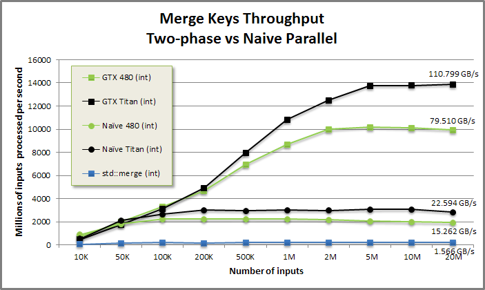
This figure benchmarks the two-phase implementation of Merge (square markers) against the naive parallel version (round markers). Due to the device's advantage in memory bandwidth, even the unoptimized GPU code beats STL by 10x (run on a Sandy Bridge i7 at 2.8ghz). The two-phase implementation beats the naive code by 5x for large inputs.

The two-phase implementation's throughput grows as the workload increases, better filling the device. The naive code hits its highest throughput for small problem sizes. While wider workloads run with better execution efficiency on the device (more concurrency means better latency hiding), this benefit is counteracted by the O(n log n) work-efficiency—the cost of the binary search grows with the log of the input size.

Two-phase design delivers consistently high throughput of merge-like functions, while promoting code reuse and readability.

From scan to load-balancing search

Most early work on GPU algorithms reduce to scan or scan-like patterns. Scan is a miracle of efficient parallel communication. Radix sort, perhaps the most successful general-purpose CS algorithm to build on GPU, is essentially a very intricate scan: because of the mechanical and regular nature of radix sort, scan manages to both evenly distribute work over threads and solve the key-ranking problem.

Conventional wisdom is to lower every problem to scan, because we've proven that scan helps solve problems with cooperative parallelism. The flaw in this reasoning is that we don't need to actually solve most problems in parallel—it is simpler and more efficient to partition problems in parallel, then solve them sequentially. Modern GPU pushes out the frontier by experimenting with new idioms and only using scan when it is the right tool for the job.

We introduce a new pattern, load-balancing search, which can be thought of as a particular type of inverse of scan. Access to this operator makes certain problems trivial and generally helps reduce the circumlocutions of scan-centric parallel programming. The load-balancing search uses two-phase decomposition to make certain dependencies explicit and further ease scheduling burdens.

Expand

Consider a vectorized fill function. It replicates each input, in order, a variable number of times. We'll call it expand.

We start with a set of input values (the alphabet) and a corresponding set of counts. Scan the counts to compute the offsets for each fill operation. Loop through the list of offsets and call std::fill to copy each input, values[i], Counts[i] times.

Thrust provides a set of primitives (transform, scan, gather, scatter, compact) that are composed with iterators, operators, and comparators to solve problems. The user typically calls transform, gather, and scatter to prepare intermediate values, scans or compacts them, and uses transform, gather, and scatter to complete the function. The difficulty is that there is no separation between two basically distinct challenges—partitioning and work logic.

thrust/examples/expand.cu

// This example demonstrates how to expand an input sequence by 
// replicating each element a variable number of times. For example,
//
//   expand([2,2,2],[A,B,C]) -> [A,A,B,B,C,C]
//   expand([3,0,1],[A,B,C]) -> [A,A,A,C]
//   expand([1,3,2],[A,B,C]) -> [A,B,B,B,C,C]
//
// The element counts are assumed to be non-negative integers

template <typename InputIterator1,
          typename InputIterator2,
          typename OutputIterator>
OutputIterator expand(InputIterator1 first1,
                      InputIterator1 last1,
                      InputIterator2 first2,
                      OutputIterator output)
{
  typedef typename thrust::iterator_difference<InputIterator1>::type
      difference_type;
  
  difference_type input_size  = thrust::distance(first1, last1);
  difference_type output_size = thrust::reduce(first1, last1);

  // scan the counts to obtain output offsets for each input element
  thrust::device_vector<difference_type> output_offsets(input_size, 0);
  thrust::exclusive_scan(first1, last1, output_offsets.begin()); 

  // scatter the nonzero counts into their corresponding output positions
  thrust::device_vector<difference_type> output_indices(output_size, 0);
  thrust::scatter_if
    (thrust::counting_iterator<difference_type>(0),
     thrust::counting_iterator<difference_type>(input_size),
     output_offsets.begin(),
     first1,
     output_indices.begin());

  // compute max-scan over the output indices, filling in the holes
  thrust::inclusive_scan
    (output_indices.begin(),
     output_indices.end(),
     output_indices.begin(),
     thrust::maximum<difference_type>());

  // gather input values according to index array
  // (output = first2[output_indices])
  OutputIterator output_end = output; thrust::advance(output_end, output_size);
  thrust::gather(output_indices.begin(),
                 output_indices.end(),
                 first2,
                 output);

  // return output + output_size
  thrust::advance(output, output_size);
  return output;
}

Counts:
    0:     3    1    0    0    7    3    2   14    4    6
   10:     0    2    1    5    3    0    5    1    6    2
   20:     0    0    9    3    2    1
   
Result of exclusive_scan:
    0:     0    3    4    4    4   11   14   16   30   34
   10:    40   40   42   43   48   51   51   56   57   63
   20:    65   65   65   74   77   79
   
Result of scatter_if:
    0:     0    0    0    1    4    0    0    0    0    0
   10:     0    5    0    0    6    0    7    0    0    0
   20:     0    0    0    0    0    0    0    0    0    0
   30:     8    0    0    0    9    0    0    0    0    0
   40:    11    0   12   13    0    0    0    0   14    0
   50:     0   16    0    0    0    0   17   18    0    0
   60:     0    0    0   19    0   22    0    0    0    0
   70:     0    0    0    0   23    0    0   24    0   25
   
Result of inclusive_scan with thrust::maximum():
    0:     0    0    0    1    4    4    4    4    4    4
   10:     4    5    5    5    6    6    7    7    7    7
   20:     7    7    7    7    7    7    7    7    7    7
   30:     8    8    8    8    9    9    9    9    9    9
   40:    11   11   12   13   13   13   13   13   14   14
   50:    14   16   16   16   16   16   17   18   18   18
   60:    18   18   18   19   19   22   22   22   22   22
   70:    22   22   22   22   23   23   23   24   24   25

Result of gather:
    AAABEEEEEEEFFFGGHHHHHHHHHHHHHHIIIIJJJJJJLLMNNNNNOOOQQQQQRSSSSSSTTWWWWWWWWWXXXYYZ

As in the CPU code, an exclusive scan converts item counts to output indices. The meaning of the rest of the implementation is somewhat obscure; I had to print the intermediate arrays to understand it. Scan is not the most natural primitive to use here, but when all you have is a hammer...

Temporary space to hold one integer per output is allocated and zeroed. scatter_if outputs the index of each input value to the start of the corresponding output run (the exclusive scan of count) if and only if the count is non-zero. Because zero counts cause consecutive output indices to match, multiple threads would attempt to store to the same address. scatter_if avoids this race condition by giving priority to the input with the non-zero count. The call to inclusive_scan specialized over the maximum functor fills the zeros with the largest indices encountered to the left. A gather loads input values at these indices and and stores them to the output, completing the expand.

Expand is a trivial function, but the use of scatter_if and inclusive_scan on maximum is far from an obvious solution. Adopting scan as the primary cooperatively-parallel function is more puzzle-solving than problem-solving. Scan is highly composable and Thrust lets you solve problems without writing new kernels. However, because you're trying to satisfy the logic of the scan function instead of targeting your specific needs, it may require non-intuitive design.

Expand with load-balancing search

MGPU introduces the Load-Balancing Search, a pattern that helps developers write elegant implementations of functions like expand. Although this search is available as a host-callable function, it is best invoked from inside a kernel. The MGPU idiom is less composable than Thrust's: users will need to write their own kernels. The solutions are much more intuitive, however, because the parallel demands of the architecture (i.e. scheduling) are satisfied in the partitioning phase, and the problem-specific logic is executed in a simple, sequential fasion. The implementation of IntervalExpand is a more direct solution to the expand problem: it loads input elements just once from global into shared memory and cooperatively fills the output arrays. The function makes only a single pass over the data and requires no auxiliary storage.

As problems become less scan-like, a gather/scatter/scan solution becomes more difficult to understand and express, and the value of composability decreases.

include/kernels/intervalmove.cuh

template<typename Tuning, typename IndicesIt, typename ValuesIt,
	typename OutputIt>
MGPU_LAUNCH_BOUNDS void KernelIntervalExpand(int destCount, 
	IndicesIt indices_global, ValuesIt values_global, int sourceCount, 
	const int* mp_global, OutputIt output_global) {

	typedef MGPU_LAUNCH_PARAMS Tuning;
	const int NT = Tuning::NT;
	const int VT = Tuning::VT;
	typedef typename std::iterator_traits<ValuesIt>::value_type T;

	union Shared {
		int indices[NT * (VT + 1)];
		T values[NT * VT];
	};
	__shared__ Shared shared;
	int tid = threadIdx.x;
	int block = blockIdx.x;

	// Compute the input and output intervals this CTA processes.
	int4 range = CTALoadBalance<NT, VT>(destCount, indices_global, sourceCount,
		block, tid, mp_global, shared.indices, true);

	// The interval indices are in the left part of shared memory (moveCount).
	// The scan of interval counts are in the right part (intervalCount).
	destCount = range.y - range.x;
	sourceCount = range.w - range.z;

	// Copy the source indices into register.
	int sources[VT];
	DeviceSharedToReg<NT, VT>(NT * VT, shared.indices, tid, sources);

	// Load the source fill values into shared memory. Each value is fetched
	// only once to reduce latency and L2 traffic.
	DeviceMemToMemLoop<NT>(sourceCount, values_global + range.z, tid,
		shared.values);
	
	// Gather the values from shared memory into register. This uses a shared
	// memory broadcast - one instance of a value serves all the threads that
	// comprise its fill operation.
	T values[VT];
	DeviceGather<NT, VT>(destCount, shared.values - range.z, sources, tid,
		values, false);

	// Store the values to global memory.
	DeviceRegToGlobal<NT, VT>(destCount, values, tid, output_global + range.x);
}

AAABEEEEEEEFFFGGHHHHHHHHHHHHHHIIIIJJJJJJLLMNNNNNOOOQQQQQRSSSSSSTTWWWWWWWWWXXXYYZ

The first half of KernelIntervalMove is boilerplate. mp_global points to coarse-grained partitioning information computed in prior to the launch. CTALoadBalance uses this to subdivide the input and output ranges into intervals that fit exactly in CTA shared memory.

CTALoadBalance fills shared memory with two non-descending sequences: references to the generating source object for each destination object (in green), and the scan of source object item counts (in black). It's not coincidence that the array of source references is exactly the same as the array of gather indices computed by Thrust's expand function. With one boilerplate call we've already solved the problem! CTALoadBalance does as much work as the scatter_if and inclusive scan on maximum, yet never has to materialize intermediates into global memory, and so requires no storage.

The kernel moves on to load the source indices into register, freeing up shared memory. It cooperatively loads the referenced source values into shared memory (the 26 letters of the alphabet). Each thread uses the source indices to gather up to VT values, then stores them to the output array. This implementation is much faster than the scan-based version using Thrust. As developers gain more exposure to the patterns involved, code written in this idiom will become easy to read and write.

Because it delivers gather indices so readily, it may seem that CTALoadBalance is just part of an expand implementation. In fact, the load-balancing search is a highly general tool. Rather than solving the expand problem, it simply partitions for this class of problems. In the case of expand, the code that is executed per work-item is trivial (we just copy from the source to the destination). Interval move (a vectorized memcpy) and relational join (including full outer join) are implemented with the same partitioning boilerplate, but with additional problem-specific logic. The load-balancing search introduces a new pattern for GPU computing, one that I hope will push out the frontier and allow users to run more ambitious calculations.

Algorithms

The algorithms in this project primarily operate on multiple sorted inputs and produce one sorted output. The collection comprises an attempt at addressing the lack of data structures on GPU. Although we don't have self-balancing trees to serve as a data store, we can use multiset union and intersection to add and remove records by key. We can use bulk insert and bulk remove for fine-grained modification of arrays given sorted indices. Vectorized sorted search is a high-throughput search with desirable work-complexity characteristics to help locate records quickly.

Although many of these functions take sorted inputs, this is not an impractical requirement. The load-balancing search pattern, introduced in the expand example, takes a sorted array, but this is typically generated by scanning a sequence of non-negative work-item counts.

Reduce and Scan - Reduce and scan are core primitives of parallel computing. These simple implementations are compact for maximum legibility, but also support user-defined types and operators.
Bulk Remove and Bulk Insert - The first routines that use coarse-grained partitioning. Remove and insert items given a sorted sequence of indices. Merge Path partitioning is introduced to serve bulk insert.
Merge - Uses Merge Path for fine-grained partitioning. The first routine that does not use scan. Develops many patterns for the routines that follow.
Mergesort - Recursively merge sorted sequences. Develops a useful and reusable CTA blocksort. Mergesort's throughput is usually beaten by radix sort for uniform random inputs, but the highly-organized structure of mergesort allows for optimizations on conditioned inputs.
Segmented Sort and Locality Sort - Segmented sort is probably the most versatile GPU sort. This allows us to sort many variable-length arrays in parallel. A list of segment head indices or an array of head flag bits is provided to define segment intervals. Segmented sort is fast: not only is segmentation supported for negligible cost, the function takes advantage of early-exit opportunities to improve throughput over vanilla mergesort. Locality sort is a useful variant that detects regions of approximate sortedness without requiring annotations.
Vectorized Sorted Search - Run many concurrent searches where both the needles and haystack arrays are sorted. This input condition lets us recast the function as a sequential process resembling merge, rather than as a traditional binary search. Complexity improves from A log B to A + B, and because we touch every input, a search can retrieve not just the lower-bound of A into B but simultaneously the upper-bound of B into A, plus flags for all elements indicating if matches in the other array exist.
Load-Balancing Search - Load-balancing search is a specialization of vectorized sorted search. It coordinates output items with the input objects that generated them. The CTA load-balancing search is a fundamental tool for partitioning irregular problems.
IntervalExpand and IntervalMove - Schedule multiple variable-length fill, gather, scatter, or move operations. Partitioning is handled by load-balancing search. Small changes in problem logic enable different behaviors. These functions are coarse-grained counterparts to Bulk Remove and Bulk Insert.
Relational joins - Sort-merge joins supporting inner, left, right, and outer variants. Uses vectorized sorted search to match keys between input arrays and load-balancing search to manage Cartesian products.
Multisets - Replace Merge Path partitioning with the sophisticated Balanced Path to search for key-rank matches. The new partitioning strategy is combined with four different serial set operations to support CUDA analogs of std::set_intersection, set_union, set_difference, and set_symmetric_difference.
Segmented reduce - .

Introduction

Libraries

Goals

Utility

Novelty

Clarity

Hackability

Two-phase decomposition

From scan to load-balancing search

Expand

Expand with load-balancing search

Algorithms